How to identify blurry images

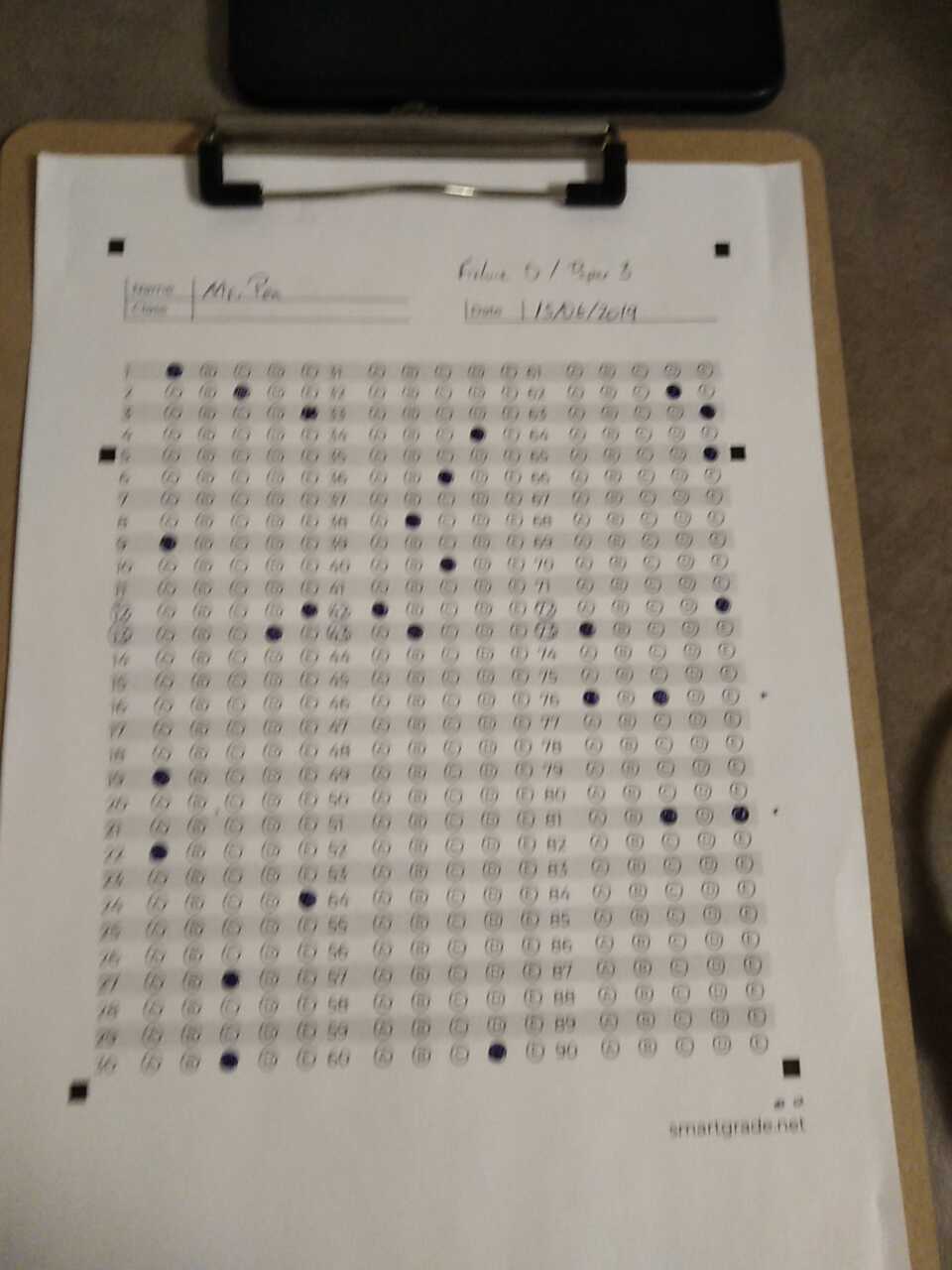
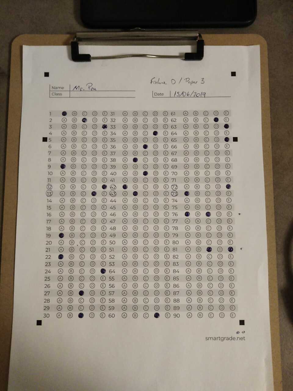
Our pair of test subjects. A blurry image on the left and a sharp one on the right

You can find the code for this post in this Jupyter notebook.

Enhance!

To make our lives easier, let’s take a look at a literally smaller problem. We’ll convert the images to grayscale and focus on a 50x50 pixels square patch from both images.

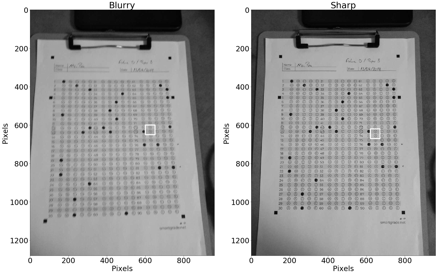
Grayscale test images

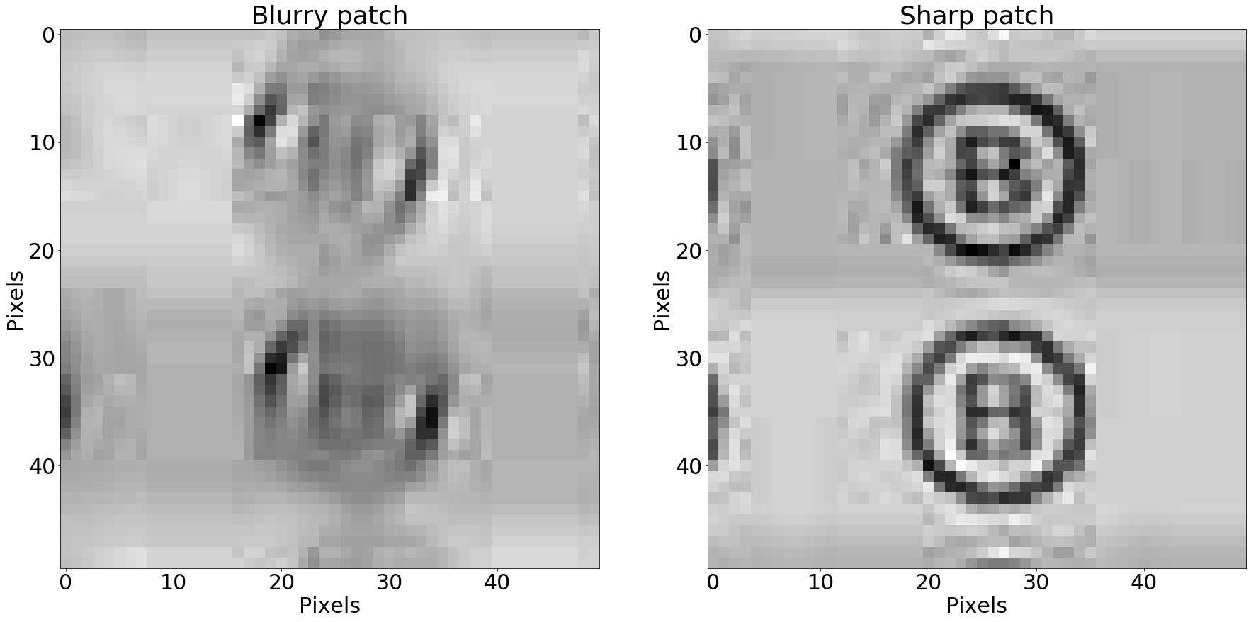
50x50 pixels square patch from both images

Zooming in makes the blurry patch look really… blurry. But how do we define our interpretation of this blurriness?

The Sobel filter

“I know!”, we might say. The edges in the blurry image are not so clear. In image processing speak, an edge is a region of quick color (or brightness in grayscale images) change. The quicker the change, the clearer, or sharper, the edge.

So, in order to find edges, we need to investigate how neighboring pixels look in comparison to each other. For instance, to find horizontal edges in an image, we might imagine ourselves walking along a row of pixels, from left to right. Whenever the next step puts us in a brighter pixel than the one before, that’s a positive change, or a positive gradient. If we go to a darker pixel, that’s a negative change, or a negative gradient. This is roughly the idea behind the Sobel filter.

Here is what our patches look after applying it in the horizontal direction:

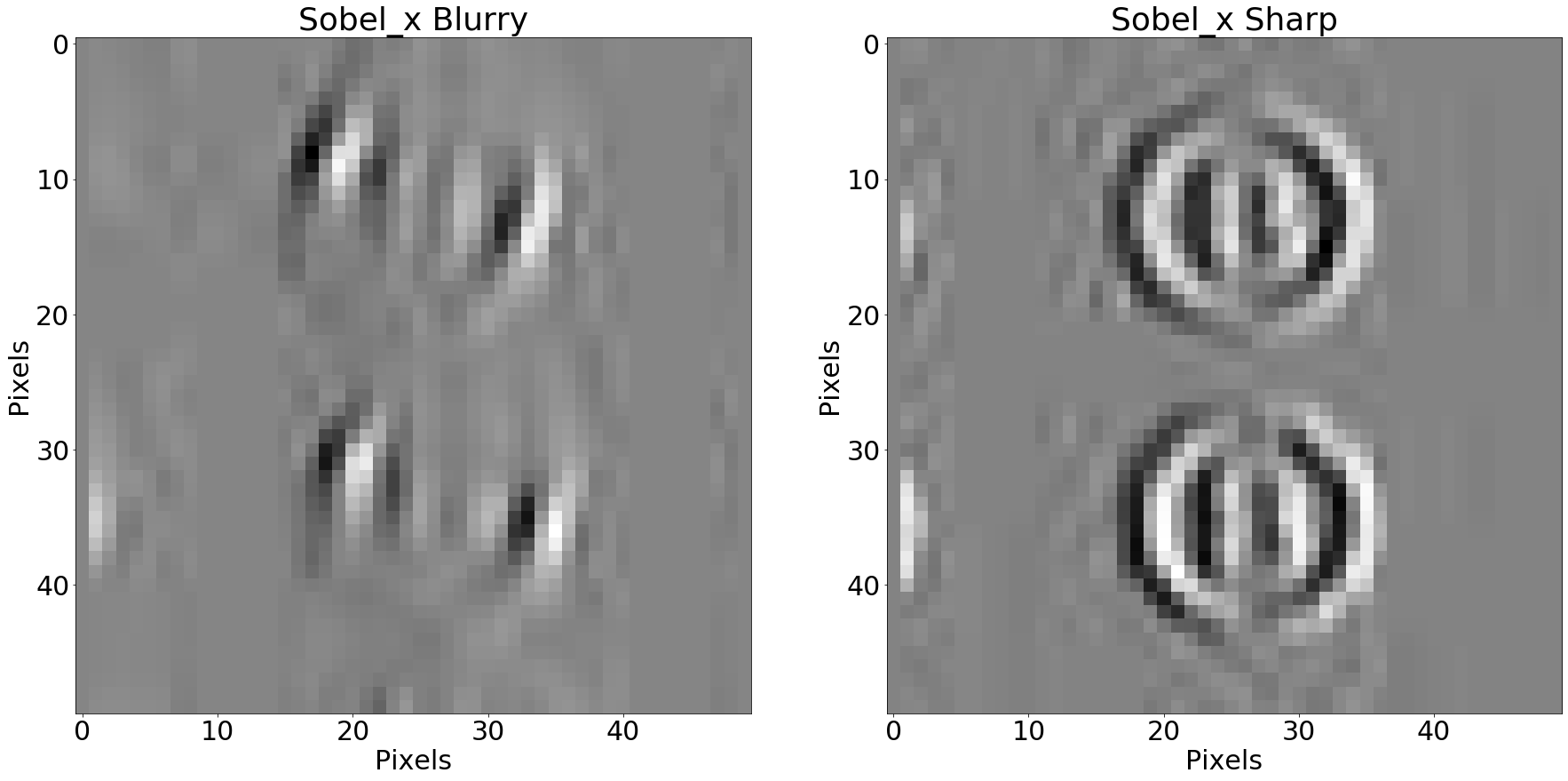
Result of applying the Sobel horizontal filter - horizontal gradient component

The patches above now represent horizontal change, or the horizontal component of the image gradient at each position in the original patches:

Darker pixels mean negative change (left neighbors are brighter than the right neighbors)
Brighter pixels mean positive change (left neighbors are darker than the right neighbors)
Grey pixels mean neighbors look roughly alike

We can do the same with the vertical Sobel filter:

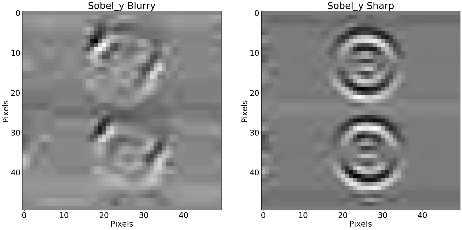
Vertical Sobel filter applied to the patches

With both the horizontal and vertical gradient components at hand, we can identify regions where the image brightness change “a lot” in either direction, either positively and negatively. In practical terms, we can combine both values for each pixel into a magnitude, a value that represents how much “change” is happening at a given pixel, regardless of direction:

def edges_magnitude(img):
  sobel_x = cv2.Sobel(img, cv2.CV_64F, 1, 0, ksize=5)
  sobel_y = cv2.Sobel(img, cv2.CV_64F, 0, 1, ksize=5)
  return cv2.magnitude(sobel_x, sobel_y)

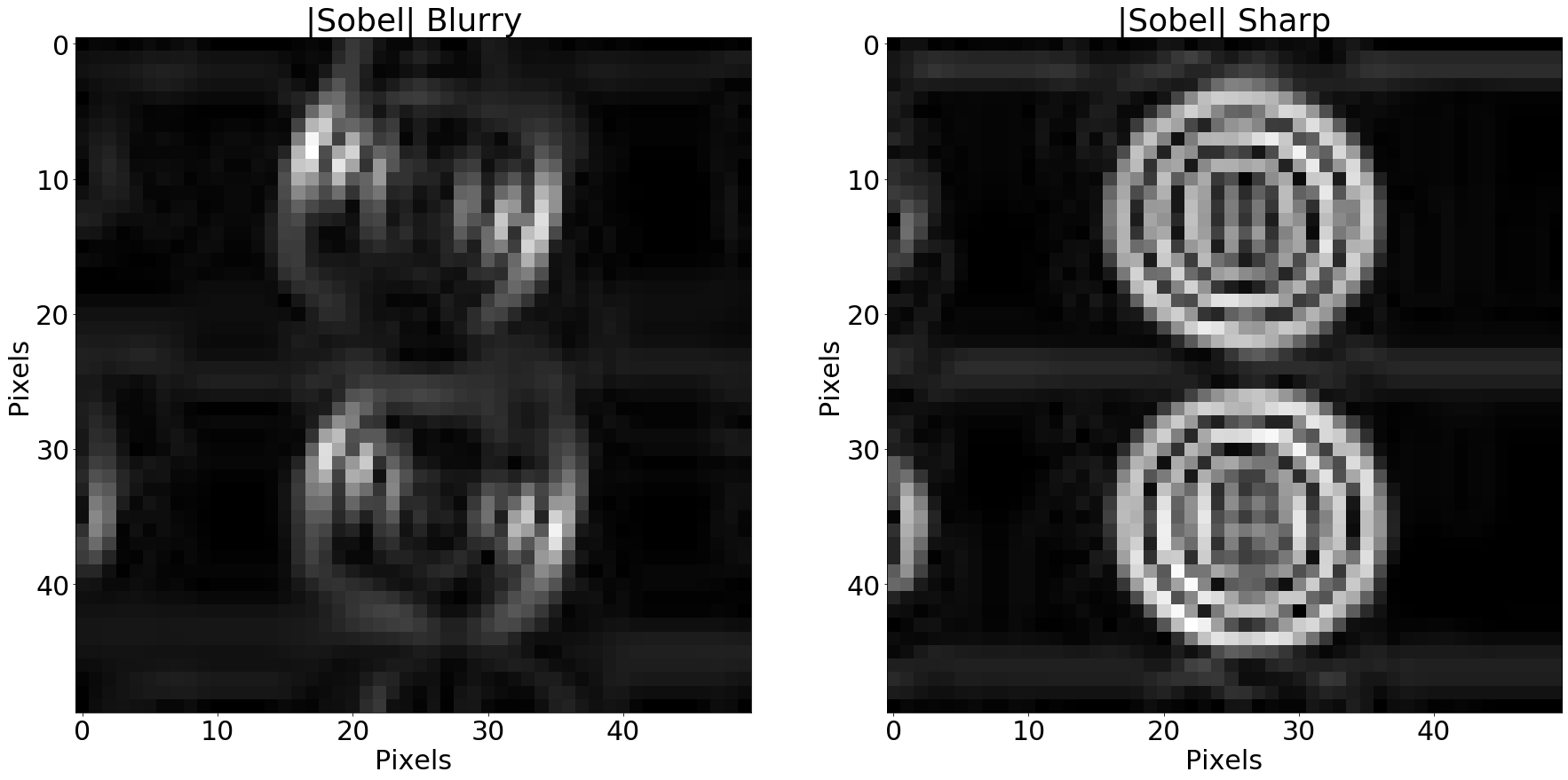
Magnitude of the Sobel gradient

Here, bright pixels represent regions of large gradient magnitudes (a lot of “change” happening). Black pixels represent regions where not much change is going on. In other words, bright pixels correspond to the edges in the original patches.

The Laplacian filter

We now know how to identify regions with edges, but how to tell wether or not they are “clear”?

In the same sense that edges represent regions of “quick change” in our image, clear edges represent areas where the edges themselves change quickly (the “gradient of the gradient”). This notion of “change of change” is captured by the Laplacian filter.

def laplacian(img):
  return cv2.Laplacian(img, cv2.CV_64F)

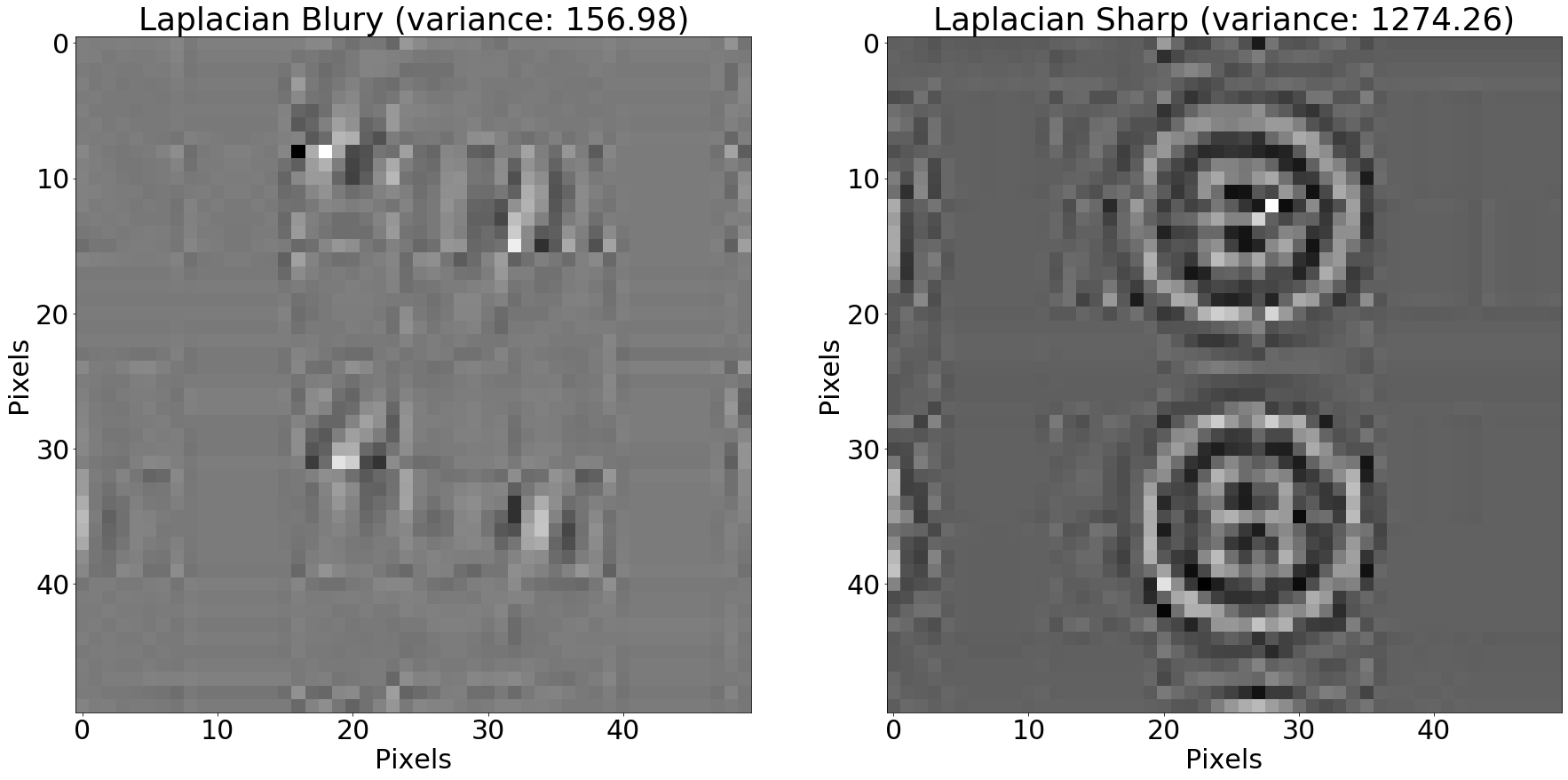
Laplacian filter applied to the patches

In the Laplacian filtered image, brighter and darker pixels represent areas where the edges change quickly (positive and negative change respectively). Gray pixels represent areas where the edges don’t change a lot.

The training set

I collected around 60 blurry and sharp pictures to make up a little training set. These images look a lot like the ones in the beginning of the post. They include some varying background, slightly different perspectives, but mostly contain the same answer sheet. If you want to play around with it, here is the tarball with the training images.

Focus measure

With the Sobel and the Laplacian filters in our toolbelt, we’re in a good position to use them as building blocks in computing different measures of how blurry an image is. The 2011 paper “Analysis of focus measure operators for shape-from-focus” present a survey of 36 (!) different techniques to measure focus on an image. I came across this paper in the great Blur detection with OpenCV article from pyimagesearch.

We’ll take a look at four different focus measure operators from the survey.

Variance of the Laplacian

As we saw, taking the Laplacian of an image highlights the pixels where the edges in the original image change quickly. Large positive values show up as white and large negative black values, as black.

Sharp images tend to have large positive and negative Laplacians. The variance of the Laplacian method explores this fact. For sharp images, the variance of the Laplacian of all pixels tend to be large. In blurry images, this value tends to be comparatively smaller, as there are less clear edges. Here’s a Python implementation using OpenCV:

def variance_of_laplacian(img):
    return cv2.Laplacian(img, cv2.CV_64F).var()

If we apply the variance of the Laplacian over our training set, we get the following plot:

Variance of the Laplacian plotted and fitted over the training data

Unfortunatelly there isn’t a nice, clear cut that divides blurry and sharp images, as we have a few sharp images with low variance. On the other hand, we have no blurry images for which the variance is above 400.

Modified Laplacian

The Modified Laplacian method explores the Laplacian operator in a different fashion. Instead of looking at the variance, it looks at the absolute values of the filtered image. The interpretation is that, in sharper images, we might see, on average, large values (both negative and positive) of its Laplacian:

def Lx(img):
  kernelx = np.array([[0, 0, 0], [-1, 2, -1], [0, 0, 0]])
  return cv2.filter2D(img, cv2.CV_32F, np.array(kernelx))

def Ly(img):
  kernely = kernelx = np.array([[0, -1, 0], [0, 2, 0], [0, -1, 0]])
  return cv2.filter2D(img, cv2.CV_32F, np.array(kernely))

def modified_laplacian(img):
  return (np.abs(Lx(img)) + np.abs(Ly(img))).mean()

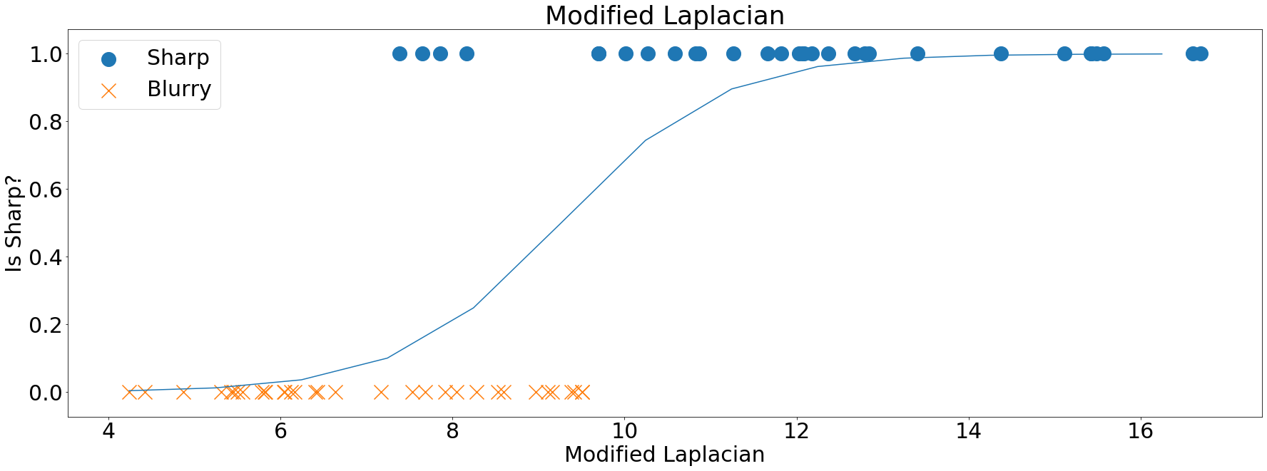
Modified Laplacian plotted and fitted over the training data

Energy of the Laplacian

The Energy of the Laplacian is fairly similar in strategy to the Modified Laplacian. It explores the fact that the Laplacian of sharp images, when squared, will produce larger values than ones from blurry images:

def energy_of_laplacian(img):
  lap = cv2.Laplacian(img, cv2.CV_32F)
  return np.square(lap).mean()

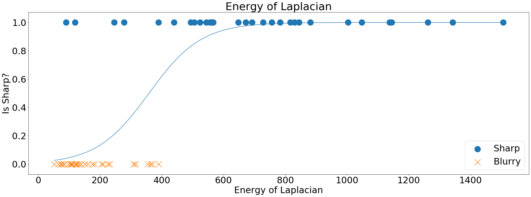
Energy of the Laplacian plotted and fitted over the training data

Tenengrad

The Tenengrad method, interestingly enough, does not rely on the Laplacian filter altogether, but on the magnitude of Sobel filter we saw earlier. If you scroll up to the image labeled “Magnitude of the Sobel gradient”, you might notice that, on the sharper image, there are more bright pixels. The Tenengrad builds on the fact that, on average, sharper images will produce larger gradient magnitudes when compared with blurry images:

def tenengrad(img):
  sx = cv2.Sobel(img, cv2.CV_32F, 1, 0, ksize=5)
  sy = cv2.Sobel(img, cv2.CV_32F, 0, 1, ksize=5)
  return cv2.magnitude(sx, sy).mean()

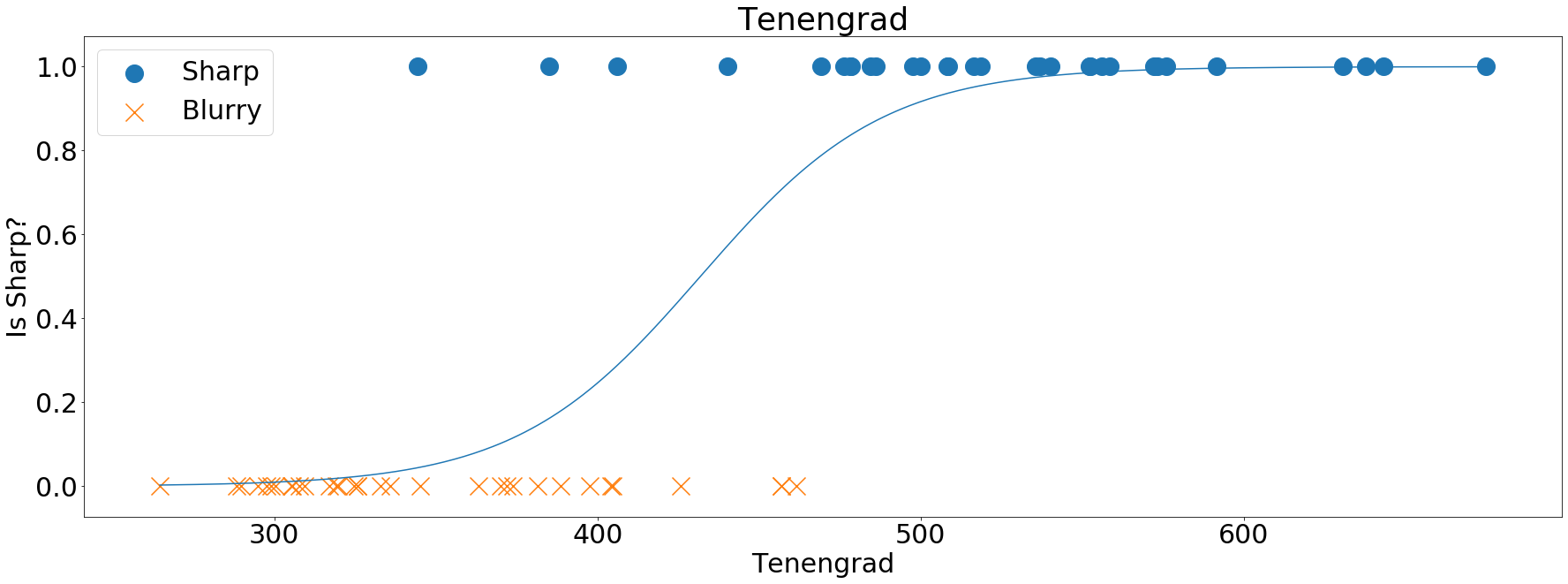
Tenengrad plotted and fitted over the training data

rbaron.net