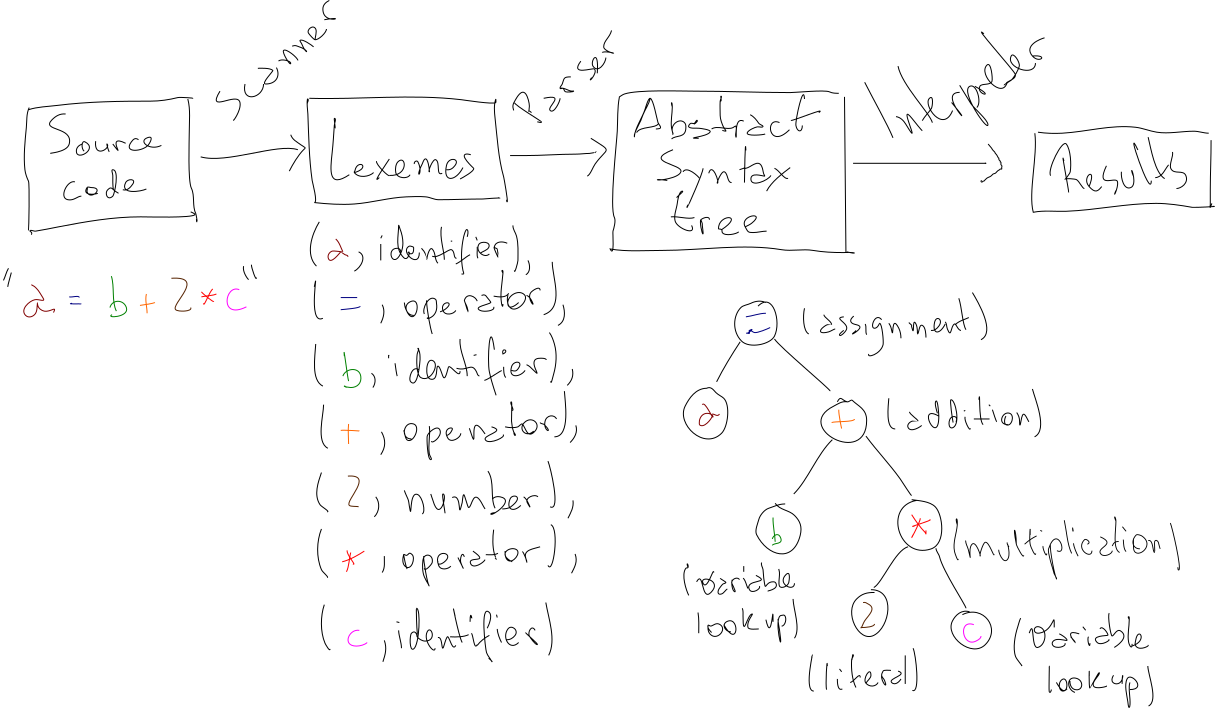
In this post, we’ll talk about a few ideas on how to build a minimal interpreted programming language from scratch, using nothing but a little theory and a little typing. We will talk about how to structure a grammar, how to build a parser and how to build an interpreter for the language we’ll design. By the end of the post, we’ll have a set of ideas and strategies for creating a weird and fun little language called No-Loop, as well as a concrete implementation for it. As a teaser, here it is in action awkwardly calculating the 6th Fibonacci number:

fib = \(n) {
  if n == 0 {
    return 0
  } else {
    if n == 1 {
      return 1
    } else {
      return fib(n-1) + fib(n-2)
    }
  }
}

// Prints to stdout
print('The result is:', fib(5)) 

Before that, though, we’ll talk about a simpler language, for which we will construct the primitives and techniques we’ll need for parsing and interpreting. This simpler language, which I called Add-Mult, handles simple integer additions and multiplications:

40 * (3 + 1 * (5 * 3))

Grammar

A grammar defines the set of valid sentences in a given language. In the context of programming languages, grammar is often part of their specifications. For instance, here’s the full grammar for Python 3.7 and here’s the analogous for ANSI C.

There is incredibly interesting theory about different types of grammars. Programming languages tend to be described using context-free grammars, a type of grammar that provides a little more expressive power than regular grammars (the type we’re more used to define through regular expressions). In practice, though, programming languages seem to incorporate constructs that slightly violate (1, 2, 3) to the context-freedom (!) of their grammar.

In order to represent a context-free grammar, the Backus-Naur form is usually employed. We’ll use it to define a tiny language that will guide us throughout this post, serving as a small starting point for the larger language we will implement:

1   <Expr> ::= <Expr> <Op> <Expr>
2           | number
3           | ( <Expr> )
4   <Op>   ::= +
5           |  *

Each line represents a production rule. Symbols surrounded by < and > are called non-terminals. Non-terminals can be further expanded by other production rules. Other values are terminals, such as number, ( or +. The | symbol separates alternatives, in such a way that <Expr> could either produce the terminal number or produce the three non-terminals <Expr> <Op> <Expr>, which can be further recursively expanded.

To get a feeling about how production rules work, let’s try to produce some strings by starting at the <Expr> (the goal) symbol:

1. <Expr> -> number (applying rule 2)

   This means that number is a valid <Expr>. Taking an instance of number, like 7, we can conclude that 7 is a valid sentence in the Add-Mult grammar.

2. <Expr> -> <Expr> <Op> <Expr> (applying rule 1)
3. <Expr> -> number (applying rule 2)
4. <Op> -> + (applying rule 4)
5. <Expr> -> number (applying rule 2)

This example shows that an expression such as `1 + 2` is a valid `<Expr>`, since we can find a sequence of production rules, starting on `<Expr>`, that will produce such an expression.

1. <Expr> -> ( <Expr> ) (applying rule 3)
2. <Expr> -> number

Through this example, we can see that expressions like ( number ) are valid <Expr>s ((42) for example).

By simply expanding non-terminals, starting with the goal symbol <Expr>, we can produce infinitely many valid sentences in the Add-Mult language. Some other examples are 1 * (2 + 3), (0) * (2 * (3 + 4)) (Can you find the sequences of production rules that would take us from an <Expr> to these examples?)

On the other hand, some invalid expressions are 1 + + 1, +, + 0, (1, since no sequence of productions rules will ever produce such sentences, no matter how hard we try.

At this point, we can generate many valid <Expr>s in the Add-Mult language just by expanding non-terminals via different production rules, just like we did in the examples above. In practice, though, we’re generally interested in the inverse problem: given a sentence and a grammar, how can we decide whether or not it is a valid sentence in the language defined by that grammar?

Top-down parsing

Given an input string and a grammar, parsing is the process of finding a sequence production rules that generates the given string. Let’s take a look at an example using our Add-Mult language and the input string 1 + 2:

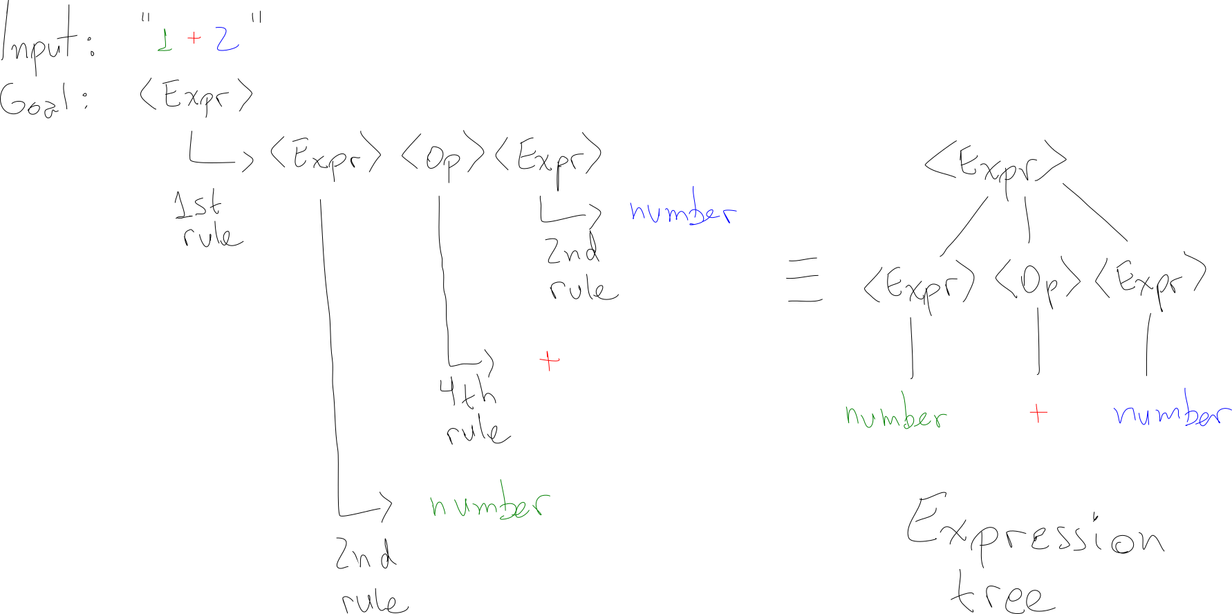
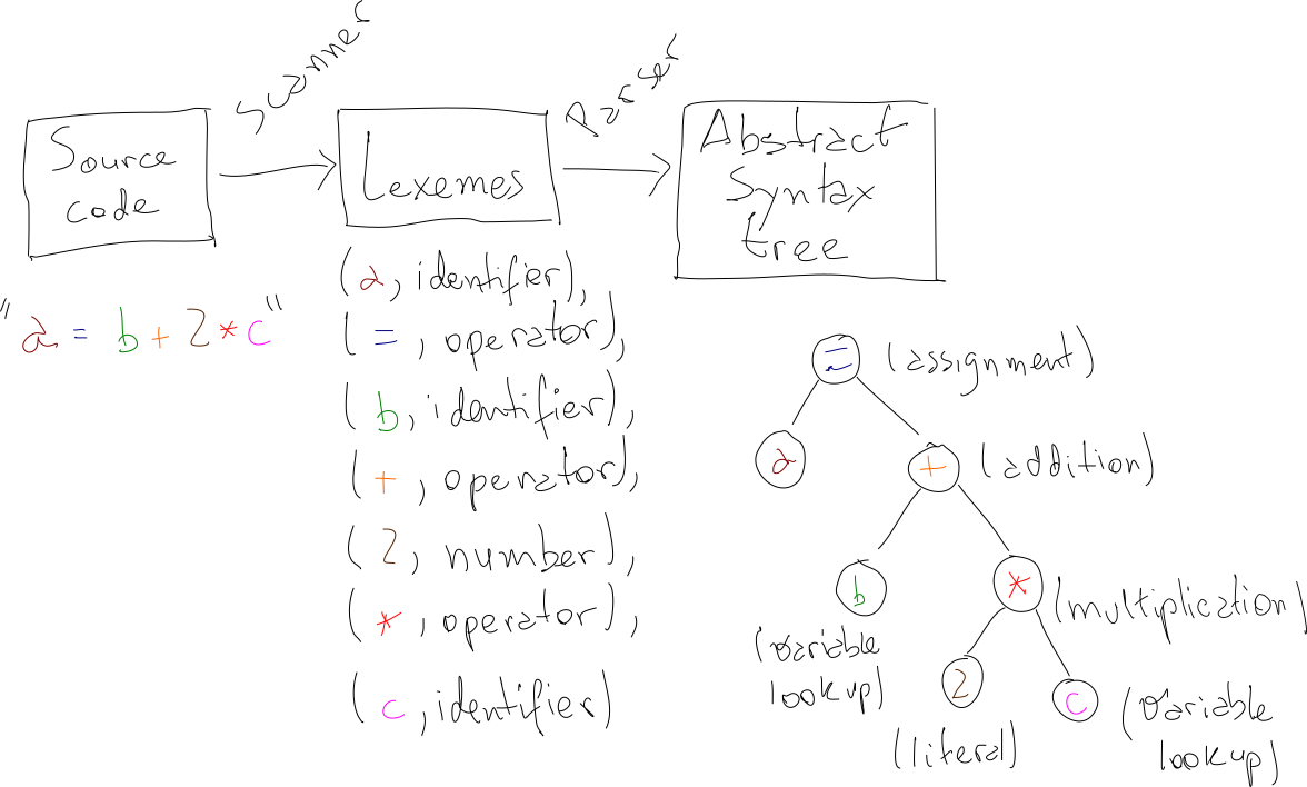
Starting at the goal non-terminal <Expr>, we can apply rules 1, 2, 4, 2, and we will find out that 1 + 2 is, indeed, a valid string in our language, since it can be derived from the starting non-terminal. If we “connect” each non-terminal to its expanded symbols, we can build a expression tree (see image above). We’ll soon discuss expression trees and related ideas further.

In this particular example, we successively applied different production rules in order to “find” the target input string. This strategy is known as top-down parsing, because we start at the root of the expression tree (the goal symbol, see image above), and we build our way down, one production rule at a time. Conversely, it is also possible to do the opposite: start with the individual terminals in the input string, and apply the production rules backwards, contracting the symbols into their original non-terminals, until we reach the goal non-terminal. This strategy is called bottom-up parsing.

Top-down parsers are easier to implement by hand, without help from parser generators such as Yacc, and that’s what we’ll do here. Simple top-down parsers are slightly more restrictive in the grammar they can handle, as we will see, but with some grammar tricks, they’re just as powerful, and are usually faster and produce more meaningful parsing errors than the automatically generated ones. As of writing, both gcc and Clang use hand-written top-down parsers.

Operator precedence

As hinted by the image above, expression trees are very closely related to the grammar specification. In fact, we’ll see it is the parser’s job to produce a nicely structured tree representation of the parsed input (according to the grammar) and hand it over to the interpreter, which will, in turn, execute it.

Informally, when producing the expression tree to be evaluated by the interpreter, the order of parsing matters. For example, we can interpret the expression 1 + 2 * 3 in two ways: (1 + 2) * 3 or 1 + (2 * 3). If we wan’t to use “regular” addition and multiplication, the latter is the correct order of evaluation. These precedence levels can be encoded in our grammar, in such a way that the produced expression tree handles precedence automatically. This is a fairly usual problem in parsing mathematical expression, and it is usually solved by the following trick: for each level of precedence, create a new non-terminal, in a way that the highest precedence expression is parsed first (that it’s further away from the root). Since we have two levels of precedence (+ and *), we can introduce the following symbols:

• <Term>s are expressions that can be be summed
• <Factors>s are expressions that can be multiplied

<Expr>   ::= <Term> + <Term>
          |  <Term>

<Term>   ::= <Factor> * <Factor>
          |  <Factor>

<Factor> ::= number
          |  ( <Expr> )

Lookahead

If we think of parsing as a search problem (“finding the sequence of production rules that takes us from the goal symbol to a given input expression”), one possible strategy is simply trying one production rule at a time and backtracking when we reach an invalid state. That is, we can exhaustively test all possible combinations of production rules, until we find a valid sequence; and if no such sequence exists, the input expression must be malformed. This works, but is prohibitively expensive: testing all possible combinations yields an exponential runtime in the size of the input expression. Even worse, we can get stuck in an infinite expansion loop, when the expansion of a production rule contains itself (such as rule 1 in the grammar above), and we’d never decide whether or not our input is parseable.

It would be great if we knew, at a given point, which production rule to expand, unambiguously. If we did, we would have no need for ever backtracking, and we could do the whole parsing by visiting each word of the input expression only once, effectively yielding a linear runtime. One usual way to achieve this goal is to keep track of the next token to be parsed, and additionally structure our grammar in a way that, looking at the next token, we can unambiguously pick up a production rule to expand.

In short, we can keep the track of the next word to be parsed, and design our grammar in a way that we can pick the next production rule just by looking at this next word. There are somewhat common tricks we can apply to our grammar to achieve that, namely left recursion removal (in order to avoid those “infinite expansion loops”) and left factoring for making sure we can unambiguously select the next production rule to expand. We can then refactor our grammar:

<Expr>   ::= <Term> <Expr'>

<Expr'>  ::= + <Term> <Expr'>
          |  $

<Term>   ::= <Factor> <Term'>

<Term'>  ::= * <Factor> <Term'>
          |  $

<Factor> ::= number
          |  ( <Expr> )

Now, let’s say we’ll start parsing with <Expr> as the goal symbol and 7 + 2 as input. With the lookahead of 1, the next token is number (the class of 7):

• <Expr> is necessarily expanded to <Term> <Expr'>
  • <Term> is necessarily expanded to <Factor> <Term'>
    • <Factor> is expanded to number (7 is consumed, now the next token is +)
    • <Term'> is expanded with $ (“empty match”, since the lookahead doesn’t match anything there)
  • <Expr'> is expanded to + <Term> <Expr'> (+ matches, so next token is now number (class of 2))
    • <Term> is necessarily expanded to <Factor> <Term'>
      • <Factor> is expanded to number (number is consumed, now the next token is $ (end of input))
      • <Term'> is expanded with $ (“empty match”, since the lookahead is the end of input)
    • <Expr'> is expanded with $ (“empty match”)

With this new version of the grammar, we can write a parser that can unambiguously choose the correct production rule to expand based solely on the next word of the to be parsed. In addition, our parser will always expand the leftmost non-terminal first. For example, if we expand <Expr> to <Term> <Expr'>, the next non-terminal to be expanded is <Term>, since it’s the leftmost one. These two characteristics make our parser a LL(1) parser: it consumes the input expression from left-to-right leftmost derivation, using at most 1 token of lookahead. That’s a mouthful, but hopefully at this point we have at least a rough idea of what these things mean.

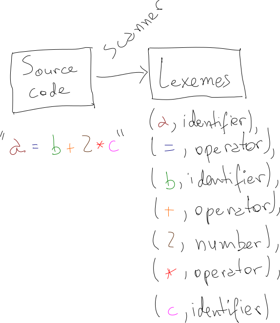
Scanner

Before getting our hands dirty with implementing the parser we designed, we should talk about scanners (also known as lexical analyzers or lexers). You may have noticed that the grammar is defined for “classes” of words. For example, our rules mention number, and not instances like 1 or 2. For our little Add-Mult language, things are pretty straightforward, but later, as we introduce more types, like string or boolean, things will get more involved.

The job of the scanner is to tag each work of the input program with a “class”.

There is also incredible theory behind scanners. The theory often touches ideas for transforming regular expressions into finite automata (e.g.: Thompson’s algorithm), so classes of words can be defined via regular expressions and recognized by the scanner. Again, there are many different “scanner generators” available, such as lex and flex.

In practice, much like parsers, many programming languages choose to implement scanners by hand, instead of relying on automatic scanners generators. For example, here’s the hand-rolled scanner for TypeScript. Here is the hand-implemented a scanner for the Add-Mult language. Given the size of the language, the code is reasonably straightforward:

def scan(string):
  lexemes = []

  pos = 0
  while pos < len(string):
      token = string[pos]

      if is_number(token):
          pos, lexeme = scan_number(string, pos)
          lexemes.append(lexeme)

      elif is_operator(token):
          pos, lexeme = scan_operator(string, pos)
          lexemes.append(lexeme)

      elif is_whitespace(token):
          pos += 1

      elif is_paren(token):
          lexemes.append(Lexeme('paren', token))
          pos += 1

      else:
          raise ValueError('Unrecognized token: {}'.format(token))

  return lexemes

Parser

Concretely, at this point, we have a LL(1) grammar for our Add-Mult language, as well as a scanner that will hand us a list of lexemes. We’re now in a good position to come up with a top-down parser that will take as input the list of lexemes and produce an expression tree. So, in addition to decide whether or not a given input is a valid sentence in the Add-Mult language, the parser will also output a representation of the source code in a convenient tree structure.

Recursive descent parsers are a type of top-down parsers that are commonly hand written. The idea is that each production rule of our grammar can be represented as a function, which takes a list of to-be-parsed lexemes and return a node of the expression tree, in a way that the set of functions can call each other mutually recursively.

We can start then by coming up with a procedure for each production rule in our Add-Mult grammar. For example, for the <Expr> and <Expr'> symbols, we can create two procedures expr and expr_prime:

def expr(stream):
    parsed_term = term(stream)
    parsed_prime = expr_prime(stream)
    return ExprNode('Expr', [parsed_term, parsed_prime])


def expr_prime(stream):
    if stream.head.value != '+':
        return None

    next(stream)
    parsed_term = term(stream)
    parsed_expr_prime = expr_prime(stream)
    return ExprNode('Expr\'', [ExprLeaf('+'), parsed_term, parsed_expr_prime])

The first version of our parser can be found here. Note that procedures call each other, so while expr can indirectly call factor, which can call expr, we won’t see an infinite loop because we structured our grammar in such a way that we can predict which production rule to expand (or which function to call) based on the next lexeme. Effectively, we have a predictive recursive descent parser.

I added a hacky support for visualizing the expression tree by outputting a DOT representation of the tree. We can use it like this:

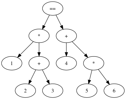
$ python expr_parser.py "(1 + 2) * 3 + 4 * ((4 * 5) + 6)" > graph.dot \
&& dot graph.dot -Tpng -o graph.png \
&& open graph.png 

Doing so will output the following image:

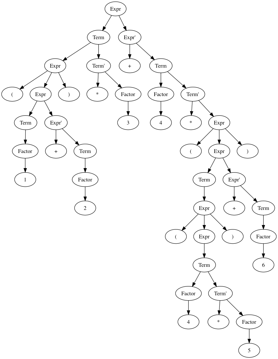
The expression tree is a great way to visualize our grammar and our parser, and make sure things look how we expect. On the other hand, it has nodes that only really exist because of the way we structured our grammar, in order to make sure precedence and lookahead are correctly handled. When we move to writing an interpreter, we won’t really care about this extra nodes. Instead of a expression tree, we can use a more compact and common representation: the abstract syntax tree.

The idea remains the same: we will come up with a (mouthful alert) predictive recursive descent parser for the grammar we designed, but we can do away with the extra nodes in the output. The functions for these extra nodes are still needed, since they dictate the order of parsing, but they don’t necessarily need to produce a node in the final tree. In short: we’ll still have the same procedures, but they’ll bypass the creation of extra nodes when possible. For example, here are the new functions for expr and expr_prime:

def expr(stream):
    parsed_term = term(stream)
    parsed_prime = expr_prime(stream)

    if parsed_prime is not None:
        return ASTNode('+', parsed_term, parsed_prime)
    else:
        return parsed_term


def expr_prime(stream):
    if stream.head.value != '+':
        return None

    next(stream)
    parsed_term = term(stream)
    parsed_prime = expr_prime(stream)

    if parsed_prime is not None:
        return ASTNode('+', parsed_term, parsed_prime)
    else:
        return parsed_term

We can now generate a abstract syntax tree for the same expression:

$ python ast_parser.py "(1 + 2) * 3 + 4 * ((4 * 5) + 6)" > graph.dot \
&& dot graph.dot -Tpng -o graph.png \
&& open graph.png 

For the same input, the abstract syntax tree representation is considerably more intelligible than the raw expression tree. Note also that the parenthesis don’t really matter after we have built the tree: the precedence is encoded in the order the nodes will be evaluated. To sum things up, here’s a diagram of our system so far:

Interpreter

With our neat abstract syntax tree in hands, it’s time to turn to evaluation. For the Add-Mult language, evaluating the tree means, informally, calculating the result of a given mathematical expression. For instance, we can say that “1 + 2” evaluates to “3”. Looking at the example AST above, we can identify two types of nodes. Intuitively, here’s how they could be evaluated:

• numbers. “1” is a valid mathematical expression whose final value is (gasp!) “1”. So numbers evaluate to themselves
• operators. A node representing + should sum the value of its left tree with the value of its right tree. Same thing for * and multiplication

That’s it. Once the parser did the heavy lifting of generating the AST, interpreting looks amazingly simple. In fact, the whole interpreter for the Add-Mult language is around 10 lines. Here’s how we can run it:

$ python interpreter.py "(1 + 2) * 3 + 4 * ((4 * 5) + 6)"
Eval'd to: 113

No-Loop

Believe it or not, in building the Add-Mult language, we touched virtually all concepts we’ll need to implement a more powerful language. We will now build upon these concepts and implement a minimal programming language, which I called No-Loop. I selected some of the most interesting topics that we’ll face when implementing support for variables, functions and extra types.

If you want to jump straight into the results, here are the goodies: grammar, scanner, parser and interpreter. Otherwise, please stick around while we talk about the ideas behind these files.

Comparisons

We can introduce comparisons to our language much like we introduces the + and * operators. The only thing we really need to think about is precedence: in which order should an expression like 1 + 2 == 3 * 1 be evaluated?

If we think about it for a while, we might realize that comparison operators (==, >= etc) should have lower precedence than mathematical expressions (the <Expr> symbols in our base grammar). Just like we dealt with precedence in our Add-Mult with <Term> and <Factor>, we can introduce a new symbol, <Comp>, that will appear higher up in our expression tree. It’s exactly the same trick:

<Comp>   ::= <Expr> <Comp'>

<Comp'>  ::= == <Expr>
          |  >= <Expr>
          |  <= <Expr>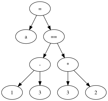
          |  $

Using this new grammar with the goal symbol <Comp>, we can implement the new comp function in our parser. At this point, we can parse expressions such as 1 * (2 + 3) == 4 + 5 * 6:

Note how the parsed tree matches our notion for operator precedence. When we later evaluate this tree in a post-order fashion, the precedence will be correct: for non-parenthesized expressions (right subtree), * nodes will be evaluated first, then +, and finally == nodes. Parenthesized expressions have higher precedence, as we can see on the left subtree ((2 + 3) will be evaluated first).

Strings

Just like numbers in the Add-Mult grammar, strings are literals: they evaluate to the value they represent: "Hello, world" is a valid No-Loop program, and it will evaluate to "Hello, world" itself. In this sense, strings and numbers have the same precedence level.

On the grammar level, we’ll need to support the string class at the same level as number. We could just extend the <Factor> symbol to do just that:

 <Factor> ::= number
           |  string
           |  ( <Expr> )

On the scanner, it’s enough to recognize the string type by identifying words starting with quotes.

Variables

Variables, from the grammar perspective, are just a new terminal: name (or identifier), and can appear wherever a literal (number or string) can appear. Whenever a name appears in an expression (other than assignment), we’ll look up the value associated with that variable and use that to evaluate the expression. For instance, in the expression a + 1, a will be looked up and it’s value will be used in place of a. We can extend the <Factor> definition with it:

 <Factor> ::= number
           |  string
           |  name
           |  ( <Expr> )

As for the interpreter, at this point, supporting variables is a matter of implementing a global environment (or scope) from which names can be looked up. In a few paragraphs, when we talk about functions, we will introduce the ability to define new environments. For now, a global environment (really a Python dict) will do. Whenever we evaluate a name, we’ll lookup that identifier on an environment and use that value to compute the evaluating expression.

Assignments

Handling assignments introduces an interesting and subtle issue. Let’s consider the expression a = 1 == 2 + 3. If we handle = as an operator, it should have lower precedence than even comparisons, since we’ll need to fully evaluate the right-hand side of the symbol = before assigning the value of a. Also, the left-hand side should be a name, since it doesn’t make much sense to do 1 = 2 + 3. With these two requirements, we may be tempted to add a new symbol potentially like the following:

<Asgn>   ::= name = <Comp>
          |  <Comp>

Since we have the the requirement that the left-hand side of = should be a name, we tentatively handled the precedence of = slightly different than the precedence for == (compare with the comparison subsection). Sadly, by introducing the name symbol in the first rule of <Asgn>, we broke the LL(1)-ness of out grammar. The reason is as follows: We’re somewhere parsing our input, and the next symbol is name. Which rule should we expand - <Asgn> or <Factor>? We just introduced ambiguity to our grammar. There are multiple ways to handle this ambiguity, like (don’t tell anyone) a little backtracking, so we could expand one of these and go back and expand the other one if it turns out it didn’t work.

A potentially simpler solution is to relax the constraints of assignments at the grammar level. If we could treat = like a regular operator (e.g.: ==, +), we know how to solve this. We can do the same precedence dance:

<Asgn>   ::= <Comp> <Asign'>

<Asign'> ::= = <Comp>
          |  $

Even though we now have an unambiguous grammar and we correctly handle the precedence of =, our grammar considers expressions like 1 + 2 = 3 to be valid. This is not very elegant, but it’s not the end of the world. We can enforce this requirement in a later time (in our case, in runtime). In fact, if we take a look at how how Python does it (if you’re brave, try to follow the expansion of the expr_stmt symbol; note that it uses the extended version of the notation we’ve been using), it seems to use a similar construct, and CPython does some special handling of assignments on the parser.

Function definitions

Inspired by Haskell’s lambda notation, I proposed the following syntax for defining anonymous functions: \(arg1, arg2) { /* function body */ } (some say that the \ symbol resembles an ASCII-friendly λ). To make named functions, we can just assign the resulting function to a variable:

increment = \(n) {
    next = next + 1
    return next
}

New symbols can be added to the grammar for handling lambda definitions. The leading \ makes it easy for us to preserve the LL(1)-ness of our grammar:

<Factor>    ::= ( <Comp> )
             |  name
             |  num
             |  string
             |  <LambDef>

<LambDef>   ::= \ <ArgsDef> { <Stmts> }

<ArgsDef>   ::= ( <ArgsNames> )

<ArgsNames> ::= name <MoreNames>
             |  $

<MoreNames> ::= , name <MoreNames>
             |  $

<Return>    ::= return <Expr>

In addition to the new <Lambdef> symbol, a few related ones were added for convenience: <Return> will instruct the interpreter to… return from the function evaluation to the original context; <ArgsDef> represents the parenthesized list of arguments names (which can be empty). <Stmts> will be explained in the following sections, but is nothing more than a sequence of statements.

Introducing function definitions bring us back to the concept of environments. Let’s take a look at the following example:

a = 1

make_inc = \(n) {
    a = n
    return \() {
      return a + 1
    }
}

// Prints 2
print(make_inc(1)())

// Prints 1
print(a)

As for the interpreter, once it finds a function definition, it will instantiate a Function object, which contains a reference to the function’s body (a list of statements) and for the enclosing environment where the function was defined:

def eval(ast, env):
    ...
    elif isinstance(ast, parser.LambDef):
        return Function(ast.args, ast.body, env)
    ...

class Function:
    def __init__(self, args, body, env):
        self.args = args
        self.body = body
        self.env = env

Function calls

Function calls take the form of print('Hello, world'). It’s a name followed by a parenthesized list of arguments. The arguments themselves can be expressions, as in f(2 * 3 + 1, a == 2). Moreover, if we want to support functions as first-class citizens, we may end up with valid code that looks like this: g()(1), if g itself returns a function.

Again, as with handling variables, we may be tempted to add a new production rule, and we will again violage the unambiguity of our grammar. This time around, though, the solution is simple, since a function call can have the same precedence level of a variable lookup. For example, in the expression: a = f(1)(2) + 3, the evaluation of f(1)(2) will have the same precedence of our literals. This means we can try to be a little clever and modify our grammar as such:

 <Factor>   ::= number
             |  string
             |  name <CallsArgs>
             |  ( <Comp> )

<CallsArgs> ::= ( <Args> ) <CallsArgs>
             |  $

<Args>      ::= <Comp> <MoreArgs>
             |  $

<MoreArgs>  ::= , <Comp> <MoreArgs>
             |  $

By introducing the <CallsArgs> symbol, which can also match an empty string, we cover both regular variables and also function calls. Note that even though we introduced another production rule starting with (, we haven’t introduced any ambiguity, since we’ll never be in a position in which we could apply both rules: expanding <CallsArgs> only happens when we’re in the middle of expanding a <Factor>.

A post on my blog wouldn’t be complete without a passionate mention to structure and interpretations of computer programs (SICP). This time, it’s nothing too philosophical, but (well now I guess it’s even worse) sort of mystical. It’s about the cover of the book:

The wizard on the left is holding a wizard thingy on which we can read “eval” and “apply” in a sort of yin-yang setting. Inside the book, the authors make the case that these are the heart and soul of interpreters, from which complex and amazing behavior arises. The eval procedure is responsible for evaluating literals, expressions, function definitions. The apply procedure executes a function, by basically calling eval on its body. Of course the body can contain function calls that apply will handle, which will cause a new function to be applied, which will… You get the idea. On our interpreter, we can do something similar: eval calls apply when it interprets a function call; apply calls eval in order to evaluate a function’s body:

def eval(ast, env):
    ...
    elif isinstance(ast, parser.FunCall):
        return apply(ast, env)
    ...

def apply(ast, env):
    fun = eval(ast.expr, env)

    args = [eval(a, env) for a in ast.args]

    # Augment function environment with arguments
    new_env = Env(fun.env, **{
        name: value
        for (name, value) in zip(fun.args, args)
    })

    return eval(fun.body, new_env)

As we talked, a function is evaluated in an environment (or scope), that contains a reference to the parent environment (where the function was original defined); this environment is initially augmented with the arguments the function were called. To get technical, this is called lexical scoping, since the scope of a function is determined by their place in the source code (and doesn’t really rely on runtime state).

As a note, we can also implement “native” functions (on the host language; Python in our case) and “install” them on our global environment. It is a matter of adding a reference to a callable in our global environment and teaching our interpreter how to apply it. Here’s the relevant part of how we can handle print.

Conditionals

Our leading Fibonacci gave us a spoiler about the syntax for handling if-then-else in our language:

if 1 == 2 {
  print('This will not be printed')
} else {
  print('This will printed')
}

For simplicity, every if must be followed by a condition (1 == 2 in our example), then by a block of code (the consequence ), then an else symbol and finally the alternative block. Handling if-else in our grammar can be done as follows:

<Stmts>     ::= <Stmt> <MoreStmts>

<MoreStmts> ::= <Stmt> <MoreStmts>
             |  $

<Stmt>      ::= <IfElse>
             |  <Return>
             |  <Asgn>

<IfElse>    ::= if <Comp> { <Stmts> } else { <Stmts> }

Now we also have a new non-terminal <Stmt> that represents statements in our grammar, consisting of either <IfElse>, <Return> or <Asgn>. If you recall, <Asgn> represents the “lower precedence” assignment operator, which actually encompasses all other precedence levels below it (comparisons, terms & factors).

The plurarized version of <Stmt> is <Stmts> and represents a sequence of statements. This is the final goal symbol for our parser: a “file” contains a list of statements; as do the alternative and consequence blocks in the if-else construct.

Next, we can add support for the if-else statement in our parser:

def ifelse(stream):
    if stream.head.value != 'if':
        return None

    next(stream)
    cond = comp(stream)

    stream.test('{')

    next(stream)
    cons = stmts(stream)

    stream.test('}')
    stream.next_and_test('else')
    stream.next_and_test('{')

    next(stream)
    alt = stmts(stream)

    stream.test('}')

    next(stream)
    return IfElse(cond, cons, alt)

As for the interpreter, evaluating an if-else node is reasonably straightforward: first, evaluate the condition. If it evaluates to a truthy value, we evaluate the consequence; otherwise we evaluate the alternative:

def eval(ast, env):
    ...
    elif isinstance(ast, parser.IfElse):
        return eval(ast.cons, env) if eval(ast.cond, env) else eval(ast.alt, env)
    ...

Examples

Even though we put in a considerable amount of work, it is still somehow mind-blowing that we’re already in a position to write reasonably useful programs in the language we designed and implemented for scratch. The no_loop/examples/ directory contains a few examples of what we can do.

Fibonacci

The Fibonacci example we saw in the beginning of the post should now work. Running this on your shell should execute the example:

$ cat examples/fib.nl
/*
 *  Calculates Fibonacci numbers
 */

fib = \(n) {
  if n == 0 {
    return 0
  } else {
    if n == 1 {
      return 1
    } else {
      return fib(n-1) + fib(n-2)
    }
  }
}

print('The result is:', fib(20))

$ python interpreter.py examples/fib.nl
'The result is:' 6765

Applying a function over a range of integers

As you may have noticed, the No-Loop language doesn’t have “while” or “for” loop statements. There isn’t a reason for this other than to keep things interesting: we’ll need recursion to achieve a similar loopy functionality (which is also a questionable choice, given we don’t do tail call optimization, but let’s not worry about it too much for this exercise). On no_loop/examples/f_range.nl we can see how to print squared and cubed integers in a given range. In your shell:

$ cat examples/f_range.nl
/*
 * Prints the result of applying a function over a range of integers
 */

square = \(n) {
  return n*n
}

cube = \(n) {
  return n*n*n
}

print_f_range = \(f, lo, hi) {
  inner = \(n) {
    if n == hi {
      return 0
    } else {
      // Print and recurse on rest
      print(f(n))
      return inner(n + 1)
    }
  }

  return inner(lo)
}

// Prints 0, 1, 4, 9, ..., 81
print_f_range(square, 0, 10)

// Prints 0, 1, 8, ... 729
print_f_range(cube, 0, 10)

$ python interpreter.py examples/f_range.nl
0
1
4
9
...
81
0
1
8
27
...
729 

Sanity-defying example: pairs and lists

Our language is very limited on the type of primitives it handles: integers and strings (booleans are sort of there too). These are all scalar types. There’s no builtin way to define composite types or lists. Or is there?

As a testament to the power of supporting functions and closures as first-class citizens, we can, amazingly, use Church pairs to emulate the behavior of heterogeneous lists. The file in no_loop/examples/pairs.nl presents a hacky implementation of pairs and lists based on this idea. Here are some interesting parts of it:

 make_pair = \(a, b) {
  // Returns a function that takes another function as argument.
  // The provided function will be applied to the original (a, b) pair
  return \(getter) {
    return getter(a, b)
  }
}

get_head = \(pair) {
  return pair(\(a, b) {
    return a
  })
}

get_tail = \(pair) {
  return pair(\(a, b) {
    return b
  })
}

// Define a pair
p1 = make_pair(1, 2)

// Prints 1
print(get_head(p1))

// Prints 2
print(get_tail(p1)) 

It doesn’t get cooler than that, does it? Doing lists this way is incredibly inefficient, since it involves multiple function calls, but the idea is just as interesting. In the next part of pairs.nl, I have built upon the concept of pairs to recursively define lists (much like list in Lisp is built on top of cons):

// Since we don't have a "null" value yet, we can improvise
// with a "sentinel". This represents the empty a list. Think of it
// as a global object (not really a list) that we convention to
// represent all empty lists.
empty_list = \() {
  return 0
}

make_range = \(lo, hi) {
  inner = \(n) {
    if n == hi {
      return empty_list
    } else {
      return make_pair(n, inner(n + 1))
    }
  }
  return inner(lo)
}

// Prints the first element of the list and recurses on the rest,
// until the list is `empty_list`
print_list = \(lst) {
  if lst == empty_list {
    return 0
  } else {
    print(get_head(lst))
    return print_list(get_tail(lst))
  }
}

// Let's create a range
range1 = make_range(0, 20)

print('Integers list:')

// Prints 0, 1, 2, ..., 19. Seriously, how cool is that?
print_list(range1)

Taking things probably too far, we can even implement the beloved map function that operates over our lists:

map = \(f, lst) {
  if lst == empty_list {
    return empty_list
  } else {
    return  make_pair(f(get_head(lst)), map(f, get_tail(lst)))
  }
}

// Prints squared numbers: 0, 1, 4, 9, 16...
print_list(map(
  \(n) { return n*n },
  make_range(0, 20)))

Exercises and food for thought

Phew! That was a lot of info, but hopefully you enjoyed reading it as much as I enjoyed writing it. I wanted to end with a few suggestions if you feel like getting your hands dirty and also a few things to think about:

• How can we support a new primitive type, like float? What rules would you add to the grammar, parser and interpreter?
• What the hell is happening with booleans? We can do 1 == 1 but there’s no true nor false values. Can you fix that?
• How can we implement while loops?
• How can we support unary operators (e.g.: -42)? What about bitwise operators? What are their precedences?
• How and when are types handled? What happens when we do 1 + 'hello, world'? When does it break?
• What about garbage collection? What’s happening right now? What if we implement a No-Loop interpreter in C?
• We implemented the map function in the examples using Church pairs. How can we implement filter?

Bugs, wrong info, questions?

Please drop me an email at rbaron <at> rbaron.net. I appreciate it!